Training MNIST with pytorch
17th Dec 2024
The Hello World Of Computer Vision
Starting from the basics, today I would like to delve into the topic of computer vision. The most well known "hello world" solved problem of computer vision is quite simple. Given greyscale images of hand drawn digits (0-9), can we build a computer system which is able to reliably decipher which digit it is?

Practical Use Case Of Such An Algorithm
While there may be many use cases for such an algorithm, possibly one of the most obvious use cases for a digit classification algorithm would be for postal routing of postcodes. If a computer is able to decipher the contents of postal addressing reliably and accurately, then the process can be completely automated.
How Can We Construct This Algorithm?
We have many different options to create this algorithm, we need something that can understand a 0 looks like an elongated circle, and that a 7 is two sticks joined together at an angle, etc.
We could hard code these rules in, but they may be subject to change. What if someone writes a 7 with a curve, or an 0 with a line in the middle? How do we reliably account for the variance in how people express their own hand writing?
Machine Learning
The problem here is that we don't want to expressly specify each rule, which may be subject to change, and may not always apply, instead we should devise some code that can learn the rules for us, this is what machine learning algorithms are for.
We will choose in this case a supervised ML algorithm. This means that the training entries have corresponding labels as shown above. The image of a seven has the corresponding label 7. This will come in handy later.
Which ML Algorithm Should We Choose?
While we have many choices here, I am going to write a neural network. Neural networks generally have the best performance for this task as seen here. In order for our solution to be competitive however, we need our error rate to be below 1%.
The Code
We start by loading in our dataset:
transform = transforms.ToTensor()

train_dataset = torchvision.datasets.MNIST(root='./data', train=True,
                                           transform=transform, download=True)
test_dataset = torchvision.datasets.MNIST(root='./data', train=False,
                                          transform=transform, download=True)

train_loader = DataLoader(dataset=train_dataset, batch_size=batch_size, shuffle=True)
test_loader = DataLoader(dataset=test_dataset, batch_size=batch_size, shuffle=False)
and then defining our model:
class SimpleMLP(nn.Module):
    def __init__(self):
        super(SimpleMLP, self).__init__()
        self.flatten = nn.Flatten()
        self.fc1 = nn.Linear(28*28, 256)
        self.relu1 = nn.ReLU()
        self.fc2 = nn.Linear(256, 128)
        self.relu2 = nn.ReLU()
        self.fc3 = nn.Linear(128, 10)

    def forward(self, x):
        x = self.flatten(x)
        x = self.fc1(x)
        x = self.relu1(x)
        x = self.fc2(x)
        x = self.relu2(x)
        x = self.fc3(x)
        return x

model = SimpleMLP()
Our first layer takes in a 28 * 28 image, and maps it to neurons in our neural network. We end up with ten output neurons, one for each digit.
Next, we define the loss and optimiser:
criterion = nn.CrossEntropyLoss()
optimizer = optim.Adam(model.parameters(), lr=learning_rate)
In this case we are using CrossEntropyLoss, this is the appropriate choice in this case, becuase CrossEntropyLoss is ideal for multi class classification problems (such as MNIST).
Next, we define our training and evaluation functions:
def train(model, loader, criterion, optimizer, device='cpu'):
    model.train()
    running_loss = 0.0
    correct = 0
    total = 0

    for images, labels in loader:
        images, labels = images.to(device), labels.to(device)

        # Forward pass
        outputs = model(images)
        loss = criterion(outputs, labels)

        # Backward and optimize
        optimizer.zero_grad()
        loss.backward()
        optimizer.step()

        running_loss += loss.item() * images.size(0)
        _, predicted = outputs.max(1)
        total += labels.size(0)
        correct += predicted.eq(labels).sum().item()

    epoch_loss = running_loss / total
    epoch_acc = correct / total
    return epoch_loss, epoch_acc
def evaluate(model, loader, criterion, device='cpu'):
    model.eval()
    running_loss = 0.0
    correct = 0
    total = 0

    with torch.no_grad():
        for images, labels in loader:
            images, labels = images.to(device), labels.to(device)
            outputs = model(images)
            loss = criterion(outputs, labels)

            running_loss += loss.item() * images.size(0)
            _, predicted = outputs.max(1)
            total += labels.size(0)
            correct += predicted.eq(labels).sum().item()

    epoch_loss = running_loss / total
    epoch_acc = correct / total
    return epoch_loss, epoch_acc
then we train and evaluate:
device = torch.device('cuda' if torch.cuda.is_available() else 'cpu')
model.to(device)

for epoch in range(num_epochs):
    train_loss, train_acc = train(model, train_loader, criterion, optimizer, device)
    val_loss, val_acc = evaluate(model, test_loader, criterion, device)

    print(f"Epoch [{epoch+1}/{num_epochs}]: "
          f"Train Loss: {train_loss:.4f}, Train Acc: {train_acc:.4f} | "
          f"Val Loss: {val_loss:.4f}, Val Acc: {val_acc:.4f}")
in this case, I opt to have it run on my GPU, since that is faster than using CPU.
Results:
Epoch [1/5]: Train Loss: 0.2817, Train Acc: 0.9200 | Val Loss: 0.1293, Val Acc: 0.9611
Epoch [2/5]: Train Loss: 0.1078, Train Acc: 0.9675 | Val Loss: 0.0995, Val Acc: 0.9692
Epoch [3/5]: Train Loss: 0.0730, Train Acc: 0.9771 | Val Loss: 0.0854, Val Acc: 0.9742
Epoch [4/5]: Train Loss: 0.0527, Train Acc: 0.9836 | Val Loss: 0.0973, Val Acc: 0.9708
Epoch [5/5]: Train Loss: 0.0407, Train Acc: 0.9872 | Val Loss: 0.0777, Val Acc: 0.9776
We were able to achive ~97% accuracy in this case, which is unfortunately not good enough. In order to have a competitive model, we need accuracy above 99%.
Improving our Model
We can however, improve our model by adding convolutional layers, the maths for convolutional layers is out of scope for this article, but more information can be found here. TLDR, convolutional layers essentially act as filters in computer vision models, allowing the model to learn how shapes form images.
We replace our MLP with a CNN:
class SimpleCNN(nn.Module):
    def __init__(self):
        super(SimpleCNN, self).__init__()
        # Convolutional layers:
        # Input: (N, 1, 28, 28)
        self.conv1 = nn.Conv2d(in_channels=1, out_channels=32, kernel_size=3, padding=1)
        self.relu1 = nn.ReLU()
        self.pool1 = nn.MaxPool2d(kernel_size=2, stride=2)
        # After first conv + pool: (N, 32, 14, 14)

        self.conv2 = nn.Conv2d(in_channels=32, out_channels=64, kernel_size=3, padding=1)
        self.relu2 = nn.ReLU()
        self.pool2 = nn.MaxPool2d(kernel_size=2, stride=2)
        # After second conv + pool: (N, 64, 7, 7)

        # Flatten the output: 64 * 7 * 7 = 3136 features
        self.fc1 = nn.Linear(64*7*7, 128)
        self.relu3 = nn.ReLU()
        self.fc2 = nn.Linear(128, 10)

    def forward(self, x):
        x = self.conv1(x)
        x = self.relu1(x)
        x = self.pool1(x)

        x = self.conv2(x)
        x = self.relu2(x)
        x = self.pool2(x)

        x = x.view(x.size(0), -1)  # Flatten
        x = self.fc1(x)
        x = self.relu3(x)
        x = self.fc2(x)
        return x
which allows us to achieve far better performance:
Epoch [1/5]: Train Loss: 0.1725, Train Acc: 0.9480 | Val Loss: 0.0570, Val Acc: 0.9811
Epoch [2/5]: Train Loss: 0.0494, Train Acc: 0.9848 | Val Loss: 0.0326, Val Acc: 0.9886
Epoch [3/5]: Train Loss: 0.0329, Train Acc: 0.9902 | Val Loss: 0.0306, Val Acc: 0.9886
Epoch [4/5]: Train Loss: 0.0256, Train Acc: 0.9917 | Val Loss: 0.0276, Val Acc: 0.9903
Epoch [5/5]: Train Loss: 0.0198, Train Acc: 0.9938 | Val Loss: 0.0256, Val Acc: 0.9908
Now we are within our 1% error rate threshold, fantastic!
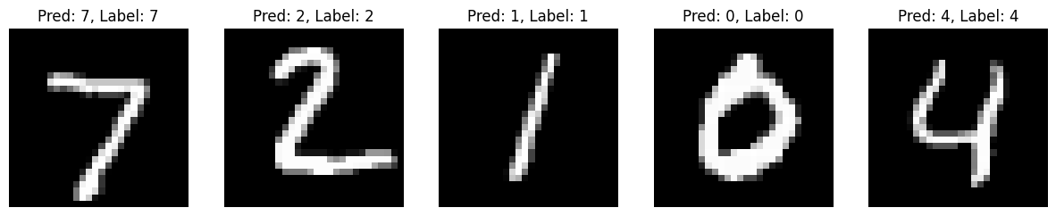
Using this code:
import matplotlib.pyplot as plt
import numpy as np

# Put the model in evaluation mode
model.eval()

# Get some examples from the test set
data_iter = iter(test_loader)
images, labels = next(data_iter)  # get a batch of images and labels
images, labels = images.to(device), labels.to(device)

# Forward pass to get predictions
with torch.no_grad():
    outputs = model(images)
    _, predicted = outputs.max(1)

# Move things to CPU for visualization
images = images.cpu()
labels = labels.cpu()
predicted = predicted.cpu()

# Visualize a few predictions
fig, axs = plt.subplots(1, 5, figsize=(15, 3))
for i in range(5):
    img = images[i].squeeze().numpy()  # shape: [1, 28, 28], squeeze to [28,28]
    axs[i].imshow(img, cmap='gray')
    axs[i].set_title(f"Pred: {predicted[i].item()}, Label: {labels[i].item()}")
    axs[i].axis('off')
plt.show()
we see that our predictions are indeed correct:
I hope this has provided insight into fundamental ML principles and shown how we can solve the MNIST problem using pytorch and neural networks, see you next time!